Reading in Data
Leslie Hendrix
August, 2020 Most of the time, you will not be hand-entering data into your R GUI. R can read datasets into its working memory that are stored in other places, such as on a hard drive or a website and it can read most any data format. In class, you will mostly be working with .csv files (comma separated values file), so this is what is covered here.
Click for Diamonds Data
These R Help pages use the “diamonds” dataset from the ggplot2 graphics package in R, by Hadley Wickham and Winston Chang
A description of the variables is below:
price price in US dollars
carat weight of the diamond
cut quality of the cut (Fair, Good, Very Good, PrReemium, Ideal)
color diamond colour, from D (best) to J (worst)
clarity a measurement of how clear the diamond is (I1 (worst), SI2, SI1, VS2, VS1, VVS2, VVS1,IF (best))
x length in mm
y width in mm
z depth in mm
depth total depth percentage = z / mean(x, y) = 2 * z / (x + y)
table width of top of diamond relative to widest point
If you have a Mac, double click the diamonds.csv file on your computer. If it opens with Excel, you are good to go. If it opens in Numbers, you must change the file association or R won’t be able to read the file in. To accomplish this:
- Select the .csv file.
- Right click and choose ‘Get Info’.
- Select Excel from the ‘Open With’ dropdown menu.
- Click the ‘Change All’ button and choose ‘Continue’.
Read in the data
R has the read.csv() function for reading data from your .csv files into your workspace. A common beginner challenge is figuring out how to find your data.
file.choose() to navigate to the file
A popular way to import data among new R users is to use the file.choose() operator inside the read.csv() function. This will produce a pop-up that allows you to search for the file and double click. On a Mac with a newer operating system, using file.choose() might return a long warning that ends in “One of the two will be used. Which one is undefined.” You can ignore this warning. Important note: R version 4.0 and higher changed the way it handles character data. Make sure to add the ‘strings=T’ argument everytime you use read.csv() so that all the code on these help pages will work.
sparkly <- read.csv(file.choose(),strings=T)
It is a good idea to ‘look’ at your data to verify it is stored properly. However, you shouldn’t print the whole object ‘sparkly’, since it will fill your console window. Use one of the following to explore the dataset:
str(sparkly) #tells you the object you named 'sparkly' is a data frame and lists each variable with the type
## 'data.frame': 53940 obs. of 11 variables:
## $ X : int 1 2 3 4 5 6 7 8 9 10 ...
## $ carat : num 0.23 0.21 0.23 0.29 0.31 0.24 0.24 0.26 0.22 0.23 ...
## $ cut : Factor w/ 5 levels "Fair","Good",..: 3 4 2 4 2 5 5 5 1 5 ...
## $ color : Factor w/ 7 levels "D","E","F","G",..: 2 2 2 6 7 7 6 5 2 5 ...
## $ clarity: Factor w/ 8 levels "I1","IF","SI1",..: 4 3 5 6 4 8 7 3 6 5 ...
## $ depth : num 61.5 59.8 56.9 62.4 63.3 62.8 62.3 61.9 65.1 59.4 ...
## $ table : num 55 61 65 58 58 57 57 55 61 61 ...
## $ price : int 326 326 327 334 335 336 336 337 337 338 ...
## $ x : num 3.95 3.89 4.05 4.2 4.34 3.94 3.95 4.07 3.87 4 ...
## $ y : num 3.98 3.84 4.07 4.23 4.35 3.96 3.98 4.11 3.78 4.05 ...
## $ z : num 2.43 2.31 2.31 2.63 2.75 2.48 2.47 2.53 2.49 2.39 ...
head(sparkly) #shows first 6 rows for all columns
## X carat cut color clarity depth table price x y z
## 1 1 0.23 Ideal E SI2 61.5 55 326 3.95 3.98 2.43
## 2 2 0.21 Premium E SI1 59.8 61 326 3.89 3.84 2.31
## 3 3 0.23 Good E VS1 56.9 65 327 4.05 4.07 2.31
## 4 4 0.29 Premium I VS2 62.4 58 334 4.20 4.23 2.63
## 5 5 0.31 Good J SI2 63.3 58 335 4.34 4.35 2.75
## 6 6 0.24 Very Good J VVS2 62.8 57 336 3.94 3.96 2.48
summary(sparkly) #gives 5 number summary plus mean for quantitative variables and first 6 levels for categorical vaiables (factors in R)
## X carat cut color clarity depth table price x
## Min. : 1 Min. :0.2000 Fair : 1610 D: 6775 SI1 :13065 Min. :43.00 Min. :43.00 Min. : 326 Min. : 0.000
## 1st Qu.:13486 1st Qu.:0.4000 Good : 4906 E: 9797 VS2 :12258 1st Qu.:61.00 1st Qu.:56.00 1st Qu.: 950 1st Qu.: 4.710
## Median :26971 Median :0.7000 Ideal :21551 F: 9542 SI2 : 9194 Median :61.80 Median :57.00 Median : 2401 Median : 5.700
## Mean :26971 Mean :0.7979 Premium :13791 G:11292 VS1 : 8171 Mean :61.75 Mean :57.46 Mean : 3933 Mean : 5.731
## 3rd Qu.:40455 3rd Qu.:1.0400 Very Good:12082 H: 8304 VVS2 : 5066 3rd Qu.:62.50 3rd Qu.:59.00 3rd Qu.: 5324 3rd Qu.: 6.540
## Max. :53940 Max. :5.0100 I: 5422 VVS1 : 3655 Max. :79.00 Max. :95.00 Max. :18823 Max. :10.740
## J: 2808 (Other): 2531
## y z
## Min. : 0.000 Min. : 0.000
## 1st Qu.: 4.720 1st Qu.: 2.910
## Median : 5.710 Median : 3.530
## Mean : 5.735 Mean : 3.539
## 3rd Qu.: 6.540 3rd Qu.: 4.040
## Max. :58.900 Max. :31.800
##
View(sparkly) #Provides a pop-up spreadhseet style view of the data, but is finicky and slow on a Mac
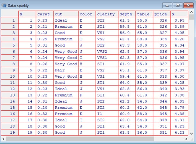
View(sparkly) on a Windows machine
If you got the above output on your R screen, you have successfully read in the data! If you would like to know how to automate the import of your data, check out the Working Directoy and Specifying the Path sections. If file.choose() works for you at this point, feel free to skip ahead to the Tips section. You can always come back later to revisit the other ways to call in data if you need it later.
Working Directory
If using file.choose() inside the read.csv() function works for youR has the concept of a working directory. If you store your data and analysis scripts there, you won’t need to point R to your file when calling it in. It will know where to look!
To find your current working directory, use the getwd() command.
getwd()
## [1] "C:/Users/leslie.hendrix/Dropbox/MGSC 291/RHelp"
This is the way a pathname looks on a Windows machine. You can see that my working directory is one of my Dropbox folders. To change the working directory to say, the desktop, change the pathname in the setwd() command. Note, if you aren’t sure of the pathname to the location you want to set, go to that location, right-click a file, choose ‘Properties’ and look at the path next to ‘Location’. Note that you must use forward slashes as separators. If you copy and paste the path and it has backslashes, you will need to change them to forward slashes.
If you use getwd() on a Mac, the pathname will look a bit different.
> getwd()
[1] “/Users/leslie.hendrix/Documents”
To find the pathname where you want to set your working directory, navigate to a file in that location and either left-click the file once and use Cmd + i or right-click and choose ‘Get Info’. The pathname is next to ‘Where:’ under general info. On my Mac, this line for a file on my Desktop says
Where: Macintosh > Users > leslie.hendrix > Desktop
Use the result from getwd() to inform you where to start in the setwd() command. You can copy and paste the path from the “where” information, but you may have to change the arrows to forward slashes if it doesn’t automatically change them for you.
> setwd(“/Users/first.last/Desktop”)
> getwd()
[1] “/Users/first.last/Desktop”
Once you have your working directory set where you want and your data saved in that location, it’s easy to call in your .csv file using the read.csv()} function and the name of the stored .csv file. Our diamonds.csv has header names, which is the default for the read.csv() function, so we can simply type the name of the file on quotes to read in the data.
sparkly <- read.csv("diamonds.csv",strings=T)
Specifying the path
You could also call the dataset in by pointing R to a specific locaton, like this on a Windows machine:
sparkly <- read.csv("C://Users/leslie.hendrix/Dropbox/MGSC 291/RHelp/diamonds.csv",strings=T)
Tips
- Make sure to give the dataset an object name. If your line of code starts with ‘read.csv’, you will print the entire dataset on your screen, which is not useful. This is the same as having it printed on a piece of paper - you won’t be able to do anything but look at it! * Use the strings=T argument everytime you use read.csv() so that all of the code on these help pages will work correctly for you.
- Notice that the dataset is called `diamonds.csv’ on your computer, but in R it is named ‘sparkly’. You can name the dataset whatever you want in R.
- Always “look” at your data after calling into R.
- If there is a space or other special character in the column name in the .csv, R will put a “.” there.
- If the column name in the .csv starts with a number, R will start that column name with an “X”.
